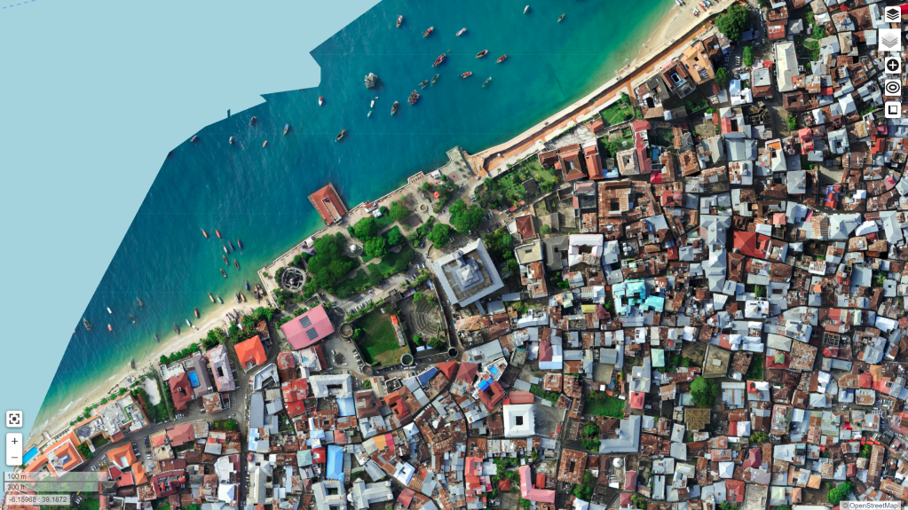
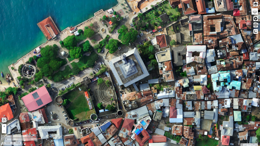
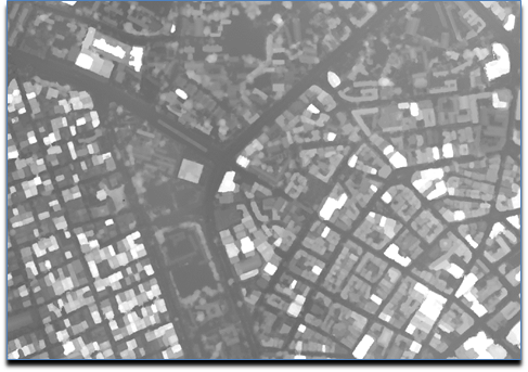
Thanks to the tireless work of the folks behind the Zanzibar Mapping Initiative, I have been exploring the latest settings in OpenDroneMap for processing data over Stone Town. I managed to get some nice looking orthos from the dataset:
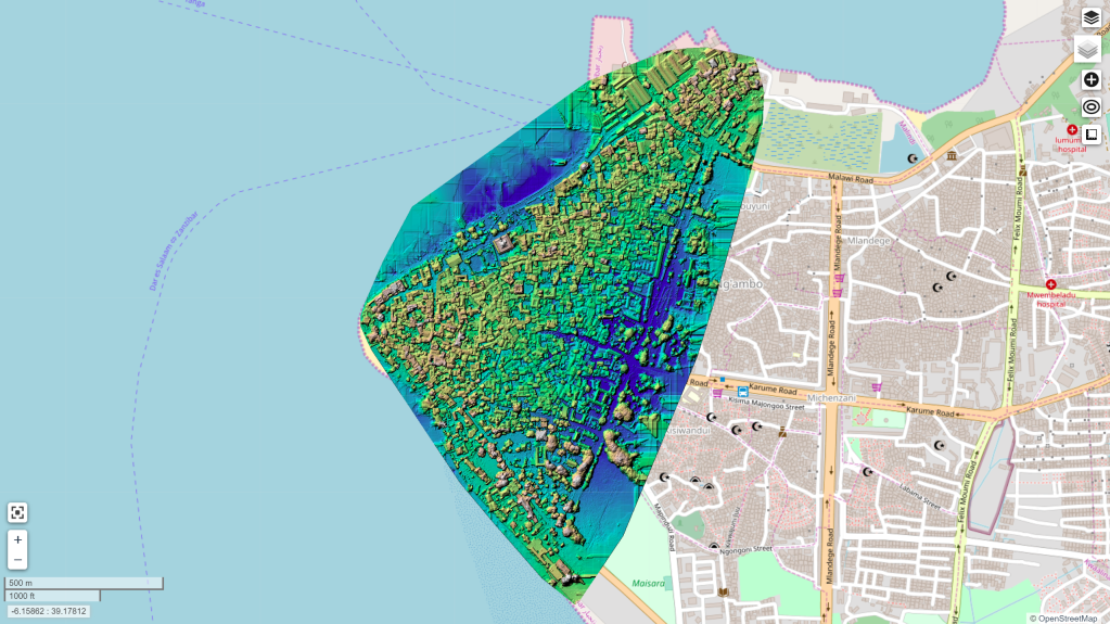
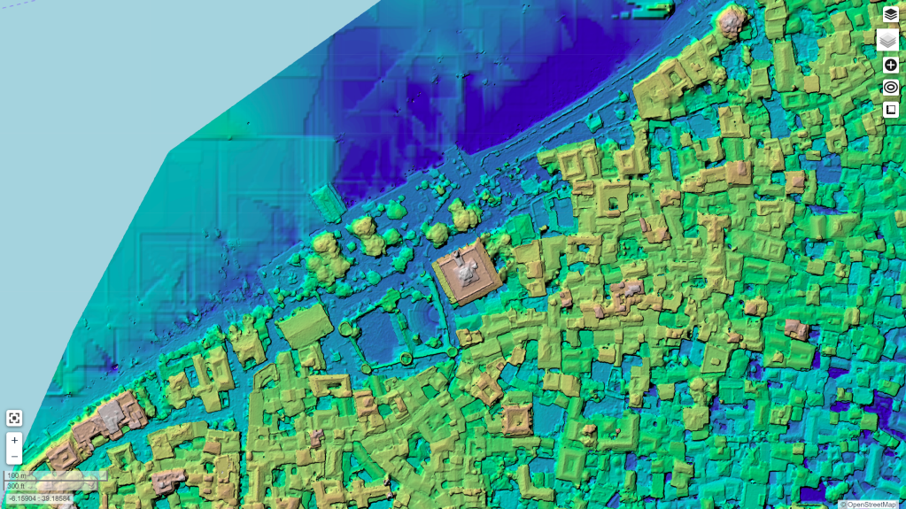
But, excitingly, I was able to extract some nice looking surface models from the dataset too. This required using the Brown-Conrady model that recently got added to OpenSfM:
This post is a small homage to the late his Majesty Sultan Qaboos. Given the strong affinity and shared history between Zanzibar and Oman, it seems fitting to post these.
In a previous blog post, we explored how we can quite effectively derive terrain models using drones over deciduous, winter scenes. We ran into some limitations in the quality of the terrain model: the challenge was removing the unwanted features (things like tree trunks) while retaining wanted features (large rock features).
I concluded the post thusly:
For our use case, however, we can use the best parameters for this area, take a high touch approach, and create a really nice map of a special area in our parks for very low cost. High touch/low cost. I can’t think of a sweeter spot to reach.
Good parameters for better filtering
In the end, the trick was to extract as good of a depthmap as possible depthmap-resolution: 1280 in my case, set the point cloud filtering (Simple Morphological Filter or SMRF) smrf-window and smrf-threshold to 3 meters to only filter things like tree trunks, and set ignore-gsd: true to ensure we are keeping the highest quality data all the way through the toolchain.
How well do the new settings work? Here’s the old vs. the new, including contours:
This is a much less noisy result. Unfortunately, I ran it at the wrong resolution, so I am rerunning at full resolution now and hope to see something similar.
From the top of Whipps Ledges at Hinckley Reservation on November 16, 2016 (Kyle Lanzer/Cleveland Metroparks)
Reposted from smathermather.com
LiDAR and photogrammetric point clouds
If we want to understand terrain, we have a pricey solution and an inexpensive solution. For a pricey and well-loved solution, LiDAR is the tool of choice. It is synoptic, active (and therefore usable day or night), increasingly affordable (but still quite expensive), and works around even thick and tall evergreen vegetation (check out Oregon’s LiDAR specifications as compared with US federal ones, and you’ll understand that sometimes you have to turn the LiDAR all the way up to 11 to see through vegetation).
For a comparably affordable solution, photogrammetrically derived point clouds and the resultant elevation models like the ones we get from OpenDroneMap are sometimes an acceptable compromise. Yes, they don’t work well around vegetation in thickets and forests, and other continuous vegetation covers, but with a few hundred dollar drone, a decent camera, and a bit of field time, you can quickly collect some pretty cool datasets.
As it turns out, sometimes we can collect really great elevation datasets derived from photogrammetry under just the right conditions. More about that in a moment: first let’s talk a little about the locale:
Sharon Conglomerate and Whipps Ledges, Hinckley Reservation
One of my favorite rock formations in Northeast Ohio is Sharon Conglomerate. A mix of sandstone and proper conglomerate, Sharon is a stone in NEO that provides wonderful plant and animal habitats, and not coincidentally provides a source of coldwater springs, streams, and cool wetland habitats across the region. A quick but good overview of the geology of this formation can be found here:
One of the conglomerate outcrops in Cleveland Metroparks is Whipps Ledges in Hinckley Reservation. It’s a favorite NEO climbing location, great habitat, and a beautiful place to explore. We wanted to map it with a little more fidelity, so we did a flight in August hoping to see and map the rock formations in their glorious detail:
Overall orthophoto of Whipps Ledges from August 2019Digital surface model of the forest overInset image of Whipps Ledges from August 2019 Inset digital surface model of the forest over
Unfortunately, as my geology friends and colleagues like to joke, to map out the conglomerate, we need to “scrape away the pesky green vegetation stuff first”. We don’t want to do this, of course — this is a cool ecological place because it’s a cool geological place! It just happens to be a very well vegetated rocky outcrop. The maple, beech, oak and other trees there take full advantage of the lovely water source the conglomerate provides, so we can’t even glean the benefits of mapping over sparse and lean xeric oak communities: this is a lush and verdant locale.
So yesterday, we flew Whipps Ledges again, but this time the leaves were off the trees. It can be a challenge still to get a good sense of the shape of the landform, even with leafless trees: forest floors do not provide good contrast with the trees above them, and it can be difficult to get good reconstructions of the terrain.
But yesterday, we were lucky: there was a thin layer of snow everywhere providing the needed contrast without being too thick to distort the height of the forest floor too much; shadows from the low sun created great textures on the featureless snow that could be used in matching.
Image above the snowy forest on Whipps Ledges
The good, the bad, and the spectacular
The bad…
So, how are the results? Let’s start with the bad. The orthophoto is a mess. There’s actually probably very little technically wrong with the orthophoto: the stitching is good, the continuity is excellent, the variation between scenes non-existent, the visual distortions minimal. But, it’s a bad orthophoto in that between the high contrast between the trees and the snow compounded with the shadows from the low, nearly cloudless sky result in a difficult to read and noisy orthophoto. Bad data for an orthophoto in; bad orthophoto out.
Orthophoto from December 21 flight
The good
The orthophoto wasn’t our priority for these flights, however. We were aiming for good elevation models. How is our Digital Terrain Model (DTM)? It’s pretty good.
Photogrammetrically derived digital terrain model from drone imagery
The DTM looks good on it’s own, and even compares quite favorably with a (admittedly dated, 2006) LiDAR dataset. It is crisp, shows the cliff features better than the LiDAR dataset, and represents the landform accurately:
Comparison of crisp and cliff-like OpenDroneMap digital terrain model and the blurry LiDAR dtm.
The spectacular
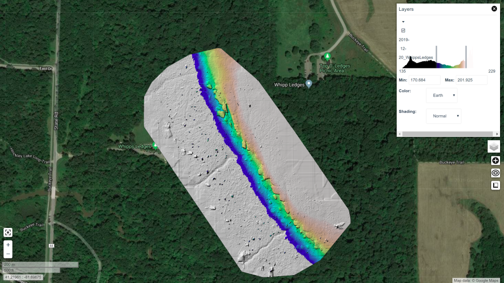
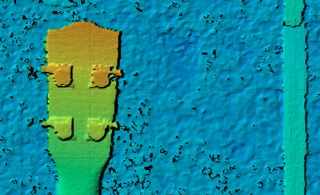
So, if the ortho is bad and the DTM is good, what is great? The DSM is quite nice:
Overview of digital Surface Model from December 21 flight
The DSM looks great. We get all the detail over the area of interest, each cliff face and boulder show up clearly in the escarpment.
Constraining the elevation range to just those elevation around the conglomerate outcrop. Constraining the elevation range to just those elevation around the conglomerate outcrop , inset 1 Constraining the elevation range to just those elevation around the conglomerate outcrop , inset 2
Improvements in the next iteration
The digital surface model is really quite wonderful. In it we can see many of the major features of the formation, including named features like The Island, a clear delineation of the Main Wall and other features that don’t show in the existing terrain models.
Due to untuned filtering parameters, we filter out more of the features than we’d like in the terrain model itself. It would be nice to keep The Island and other smaller rocks that have separated from the primary escarpment. I expect that when we choose better parameters for deriving the terrain model from the surface model points, we can strike a good balance and get an even better terrain model.
Animation comparing digital surface model and digital terrain model showing the loss of certain core features to Whipps Ledges due to untuned filtering parameters in the creation of the terrain model.
Beating LiDAR at it’s own game
It is probably not fair to say we beat LiDAR at it’s own game. The LiDAR dataset we have to compare to is 13 years old, and a lot has improved in the intervening years. That said, with a $900 drone, free software, 35 minutes of flying, and two batteries, we reconstructed a better terrain model for this area than the professional version of 2006.
And we have control over all the final products. LiDAR filtering tends to remove features like this regardless of point density, because The Island and similar formations are difficult to distinguish in an automated fashion from buildings. Tune the model for one, and you remove the other.
For our use case, however, we can use the best parameters for this area, take a high touch approach, and create a really nice map of a special area in our parks for very low cost. High touch/low cost. I can’t think of a sweeter spot to reach.
I had an interesting question recently at a workshop: “What parameters do you use for OpenDroneMap?” Now, OpenDroneMap has a lot of configurability, lots of different parameters, and it can be difficult to sift through to find the right parameters for your dataset and use case. That said, the defaults tend to work pretty well for many projects, so I suspect (and hope) there are a lot of users who never have to worry much about these.
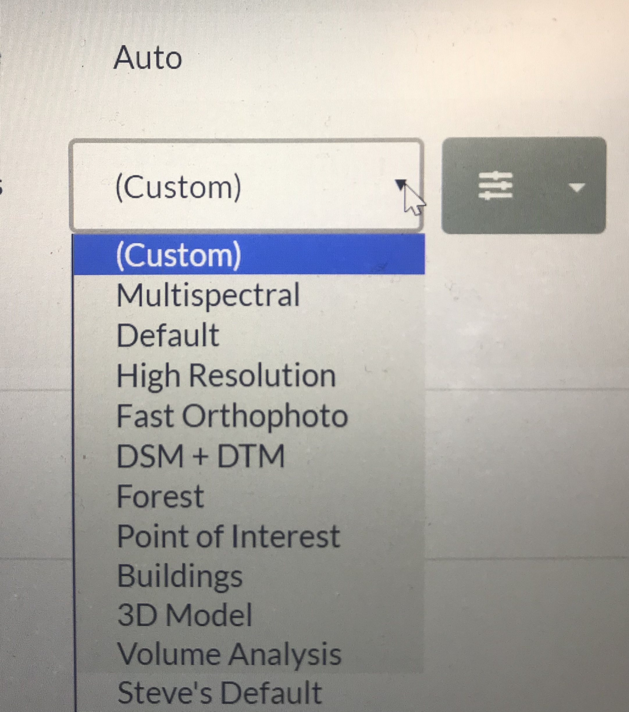
The easiest way to proceed, is to use some of the pre-built defaults in WebODM. These drop downs let you take advantage of the combination of a few different settings abstracted away for convenience, whether settings for processing Multispectral data, doing a Fast Orthophoto, flying over Buildings or Forest, etc.
You can also save your own custom settings. You will see at the bottom of this list “Steve’s Default”. This has a lot of the settings I commonly tweak from defaults.
Back to the question at hand: what parameters do I change and why? I’ll talk about 7 parameters that I regularly or occasionally change.
The Parameters
Model Detail
Occasionally we require a little more detail (sometimes we also want less!) in our 3D models from OpenDroneMap. Mesh octree depth is one of the parameters that helps control this. A higher number gives us higher detail. But, there are limits to what makes sense to set for this. I usually don’t go any higher than 11 or maybe 12.
Elevation Models
DTM/DSM
Often with a dataset, I want to calculate a terrain model (DTM) or surface model (DSM) or both as part of the products. To ensure these calculate, we set the DTM and DSM flags. The larger category for DTM and DSM is Digital Elevation Model, or DEM. All flags that affect settings for both DTM and DSM are named accordingly.
Ignore GSD
OpenDroneMap often does a good job guessing what resolution our orthophoto and DEMs should be. But it can be useful to specify this and override the calculations if they aren’t correct. ignore-gsd is useful for this.
DEM Resolution
DEM Resolution applies to both DTMs and DSMs. A criterion that is useful to follow for this setting is 1/4th the orthophoto resolution. So, if you flew the orthophoto at a height that gives you 1cm resolution ortho imagery, your dem-resolution should probably be 4cm.
Depthmaps
Depthmap resolution
A related concept is depthmap resolution. Depthmaps can be thought of as little elevation models from the perspective of each of the image pairs. The resolution here is set in image space, not geographic coordinates. For Bayer style cameras (most cameras), aim for no more than 1/2 the linear resolution of the data. So if your data are 6000×4000 pixels, you don’t want a depthmap value greater than 3000.
That said, usually, 1/4 is a better, less noisy value, and depthmap calculations can be very computationally expensive. I rarely set this above 1024 pixels.
Camera Lens Type
I saved the best for last here. So, if you’ve made it this far in the blog post, this is the most important tip. In 2019, OpenSfM, our underlying Structure from Motion library, introduced the Brown-Conrady camera model as an option. The default for camera type is auto, which usually results in the use of a perspective camera, but Brown-Conrady is much better. Set your camera-lens to brown, and you will get much better results for most datasets. If it throws an error (which does happen with some images), just switch it back to auto and rerun. Brown will be a default in the near future.
(Reposted from https://smathermather.com/2019/12/02/self-calibration-of-cameras-from-drone-flights-part-3/)
I have been giving a lot of thought to sustainable ways to handle self calibration of cameras without undue additional time added to flights. For many projects, I have the luxury of spending a little more time to collect more data, but for larger projects, this isn’t a sustainable model. In a couple of previous posts (this one and this one), we started to address this question, pulling from the newly updated OpenDroneMap docs to highlight the recommendations there.
As I have been thinking about these recommendations, there are other more efficient ways to accomplish the same goal. Enter the calibration flight: the idea is that with some cadence, we have dedicated flights at the same height and flight speed as the larger flight in order to estimate lens distortion.
INITIAL TEST
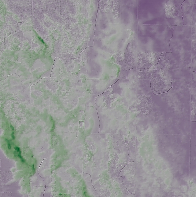
For this testing, I chose a relatively flat but slightly undulating area in Ohio in the USA: the Oak Openings region, which is a lake bottom clay lens overlayed with sand dunes from glacial lakes. It has enough topography to be interesting, but is flat enough to be sensitive to poor elevation models.
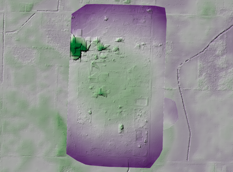
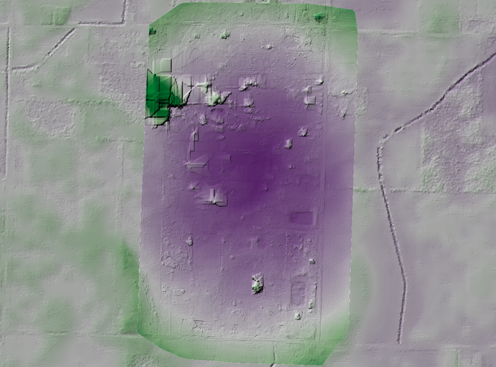
Shaded elevation model of the Oak Openings region in Northwest Ohio, USA. Purple is lower elevations, green higher elevations, typically vestigial dunes. Elevation model from Ohio Statewide Imagery Program.
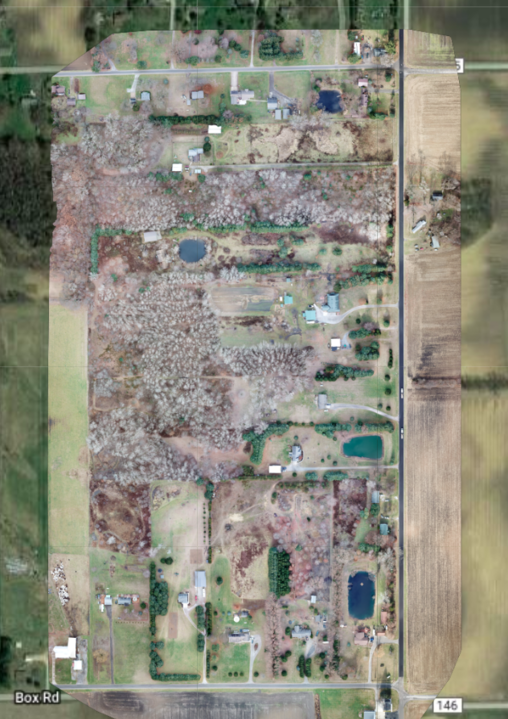
The test area flown is ~80 acres of residences, woodlots, and farmland.
80 acre aerial image
Flown with a DJI Mavic Pro which has an uncalibrated lens with movable focus, the first question I wanted to address is how much distortion do we get in our resultant elevation models if we just allow for self calibration? It turns out, we get a lot:
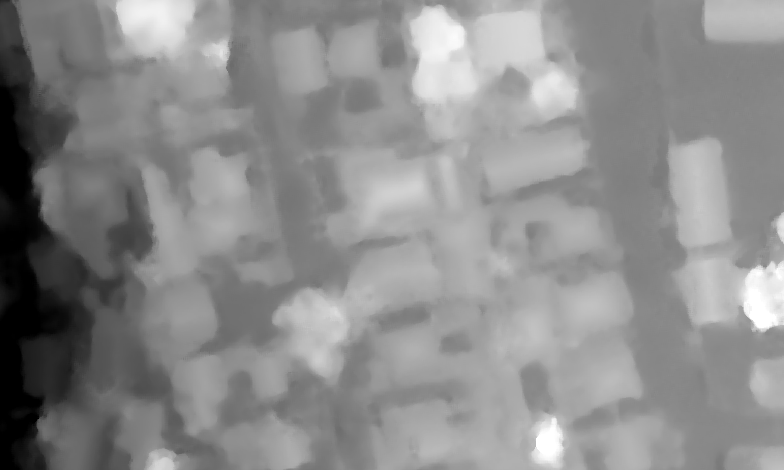
Bulls-eye pattern of lens distortion in digital terrain model with self calibrated approach
We have seen this in other datasets, but this forms a good baseline for our subsequent work to remove this.
Next step, we fly a calibration pattern. In this case, I plotted an area large enough to capture two passes of data, plus an orbit around the exterior of the area with the camera angled at 45° for a total of 3 minutes and 20 seconds.
Layout of calibration flight pattern
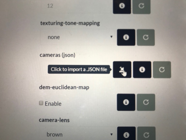
When we process this data in OpenDroneMap, we can extract the cameras.json file (either in the processing directory or we can download from WebODM) and use that in another model. We can do this using the cameras parameter on the command line or in WebODM through uploading the json file from our calibration dataset.
Cameras option in WebODM for importing camera parameters
But, before we do that, let’s do a review of our calibration data — process it and take a look at what kind of output we get. First, we process it using defaults and evaluate the elevation model to look for artifacts that might indicated whether the calibration pattern wasn’t successful.
Our terrain model from the Ohio Statewide Imagery Program elevation model looks like this for our calibration area:
Shaded elevation model from Ohio Statewide Imagery program for calibration area
Note that this is mostly a moderately flat farm field with a road and small ditches running North/South in the west of the image and a deep Northeast Ohio Classic ditch in the east.
How does our data from our calibration flight look?
Elevation model from calibration flight
It’s not bad. We can see the basic structure of the landscape — from the road in the west to the gentle drop in elevation in the east.
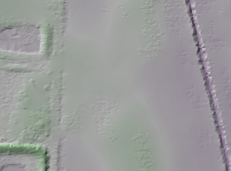
Our default camera model is a perspective camera. How does this look with the Brown–Conrady camera model that Mapillary recently introduced into OpenSfM?
Elevation model from calibration flight with Brown–Conrady camera model
With the Brown–Conrady camera model, we see additional definition of the road bed, ditches alongside the road, and even furroughs that have been ploughed into the field. For this small area, it appears the Brown–Conrady camera model is really improving our overall rendering of the digital terrain model, likely as a result of an improved structure from motion product. We even see the small rise in the field at the southern central part of the study area, and as with the default (perspective) model, the slope down toward the ditch on the east of the study area.
RESULTS
With running these both with perspective and Brown–Conrady cameras, we can apply those camera models as fixed parameters for our larger area and see what kind of results we get.
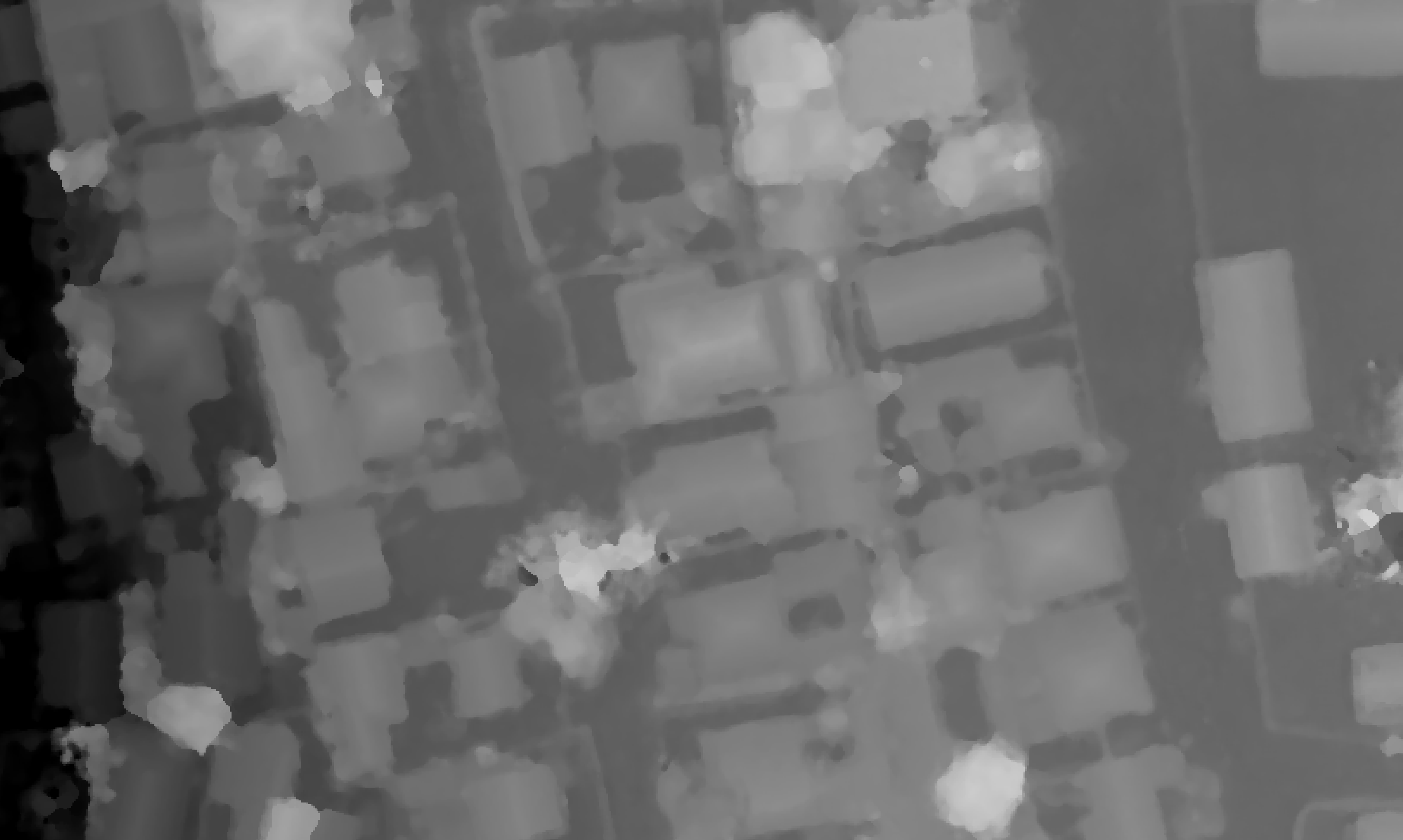
Larger elevation model as processed with perspective camera parameters as compared with reference model
Our absolute values aren’t correct (which we expect), but the relative shape is — the dataset is now appropriately relatively flat with clear delineation of some of the sand features. This is the goal, and we have achieved it with some of the most challenging data.
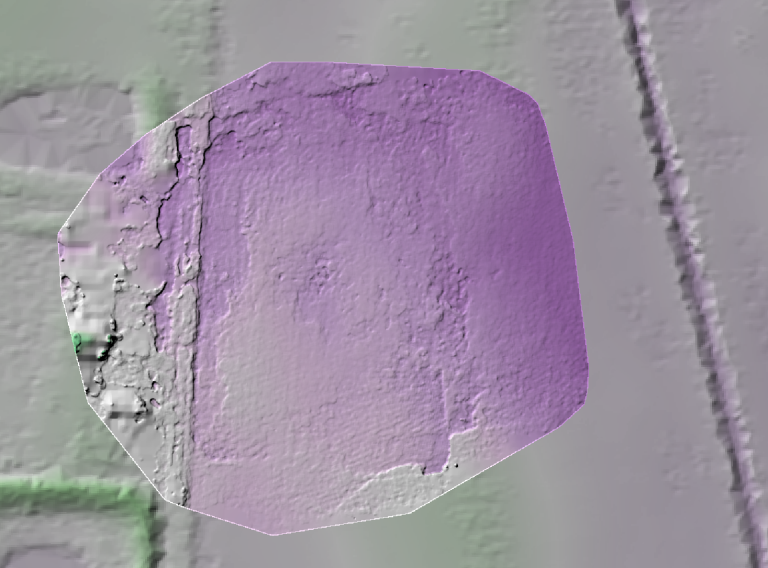
How does our Brown–Conrady calibration model turn out? It did so well on the small scale, will we see similar results over the larger area?
Larger elevation model as processed with Brown–Conrady camera parameters
In this case, no: the Brown–Conrady model over compensates for our distortion parameters. More tests need to be done in order to understand why. For now, I recommend using the perspective model for corrections on large datasets, and Brown–Conrady camera model on smaller datasets where the details matter, but the distortion isn’t discernible.
Recent posts have detailed the improvements in the digital elevation products from OpenDroneMap that are forthcoming, and we are really excited about those.
That code is now relatively mature and likely usable for your use case, with only a couple of caveats:
The first caveat is that the processing for point clouds takes 3-4 times as long. That said, the quality is so much better, I feel comfortable with calling that a feature, not a bug.
The other caveat is that the code doesn’t yet respect the “–max-concurrency” parameter. It will use every processor you have, whether you want it or not. We will be fixing that before we merge it in with the master branch.
Those caveats aside, the quality of what we get in an elevation model is almost incomparable, and the memory footprint for the dense point cloud step that we improved is 60% what it was, so processing larger datasets should become easier. Finally, while better and more detailed, the total number of points in the point clouds is decreased (about 1/3 to 1/4 the size), which may help the speed of subsequent steps, although I will confess this is an untested theory. Interestingly, even though there are fewer points, they are better distributed, so it looks like more points.
Ok, so far what is available is broken code but that will be fixed. You can check it out in the meantime in this pull request. It calculates the full depthmaps, but does not yet write the PLY file needed for subsequent steps.
The trick to improve DEMs was already in our build process: for elevation models, MVE’s dmrecon utility is a slower but otherwise better option than smvs, the utility we are currently using. It provides more detail, is less “melty” as one person described smvs to me, and overall gives us much better results. A theoretical disadvantage is that svms can find results where there aren’t features, and thus does better gap filling. For drone mapping use cases, however, this remains predominantly a theoretical and not practical limitation.
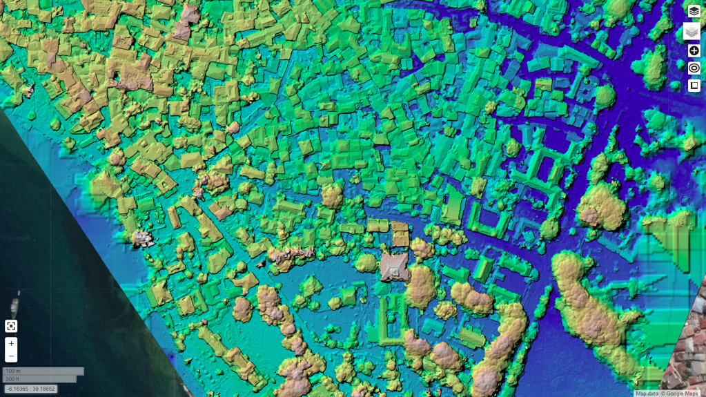
We have some cool new-to-us approaches in the works for digital elevation models. Here’s a quick teaser and comparison old to new. This is a digital surface model over some buildings, fences, and trees in Dar es Salaam:
Water running downhill is a challenge for elevation models derived from drone imagery. This is for a variety of reasons, some fixable, some unavoidable. The unavoidable ones include the challenges of digital terrain models derived from photogrammetric point clouds, which don’t penetrate the way LiDAR does. The avoidable ones we seek to fix in OpenDroneMap.
Animation of flow accumulation on poorly merged terrain model, credit Petrasova et al, 2017
The fixable problems include poorly merged and misaligned elevation models. Dr. Anna Petrasova’s GRASS utility r.patch.smooth is one solution to this problem when merging synoptic aerial lidar derived elevation models with patchy updates from UAVs.
Another fix for problematic datasets is built into the nascent split-merge approach for OpenDroneMap. In short, that approach takes advantage of OpenSfM’s extremely accurate and efficient hybrid structure from motion (SfM) approach (a hybrid of incremental and global SfM) to find all the camera positions for the data, and then split the data into chunks to process in sequence or in parallel (well, ok, the tooling isn’t there for the parallel part yet…). These chunks stay aligned through the process, thus allowing us to put them back together at the end.
For a while now, we’ve been in the awkward position with respect to the nickname: split-merge. It lacks a lot of merge features. You can merge the orthos with it, but not the remaining datasets. And while this will be true for a while longer, we have been experimenting a bit with the merging of these split datasets (thanks to help from Dr. Petrasova). Here for your viewing pleasure is the first merged elevation model from the split merge approach:
Digital surface model of Dar es Salaam, merged from 4 separately processed split-merge submodules.